
Part 2 -- Arrays, Math, and Plotting in Python
Objectives
Here we will be exploring two external libraries in Python, NumPy (Numerical Python) and Matplotlib (a plotting library that uses a number of conventions common in MATLAB).
We will mostly be using these tools to further play with our Pi script, and ending by plotting values of $\pi$ against the number of iterations (or Reimann sums) used to calculate our values.
Libraries in Python
Python is widely used and as a consequence it has accrued a large number of support libraries of functions and resources. Some are very highly specialized. Others are sufficiently generalized to have developed wide use. Some are also integerated into more specir
Today we will work with two libaries that are useful in general computation and in looking at those compitations.
- NumPy: a library that includes support for arrays, matrices, and high-level math functions.
- Matplotlib: a useful 2-d plotting library.
Accessing Libraries
There are three common ways that people access these libraries. In my scripts I prefer to put all of my called libraries towards the top of the program. Other people put them in whenever they need them.
Loading EVERYTHING in a Library and Putting it on the Same Plate as Everything Else.
In this option, you simply make all the contents of a library. Functions called from these libraries later in the program or script will not not be explicitly noticable as being taken from any given external library (which is one reason I avoid this method). The syntax for this is
##########################################################
###
### Call the the library "myLibrary"
###

from myLibrary import *

### Execute the Item from myLibrary called myFunction

myAnswer = myFunction( myArgument) )

###
##########################################################
Load a Single Element From a Library and Put it on the Same Plate as Everything Else
If you only one one or two items from the library and know you won't ask for more. You can use this function.
##########################################################
###
### Call the the library "myLibrary" and
###    ONLY get the functions myFunction and
###    myOtherFunction

from myLibrary import myArgument, myOtherArgument

### Execute the Item from myLibrary called myFunction

myAnswer = myFunction( myArgument) )

myAnswer = myFunction( myOtherArgument) )

###
##########################################################
Loading a Library and Putting it in it's own Bento Box Compartment.
You can also load a library so that all elements of a library can be accessed and so that you can see from what library it's being called from. This one is my prefered method since it makes it clear through the code that the functions or other elements of a library are needing to be brought in from the outside.
##########################################################
###
### Call the the library "myLibrary" to be sourced
###   with a reference to the library
###

import myLibrary

### Execute the Item from myLibrary called myFunction

myAnswer = myLibrary.myFunction(myArguments)

###
##########################################################
or you can shorthand the name of the library with an "alias." I personally like this one best.
##########################################################
###
### Call the the library "myLibrary" to be sourced
###   with a reference to the library
###

import myLibrary as myL

### Execute the Item from myLibrary called myFunction

myAnswer = myL.myFunction(myArguments)

###
##########################################################
Calling the Libraries we'll use today
So let's get started and load the libraries we are going to use today.
Notice the call to matplotlib (that's our graphing library). The pyplot is a sublibrary that emulates some handy Matlab plot functions. They are very popular in scientific python use and many libraries that do specialized work for a given discipline are built to leverage matplotlib.pyplot.
##########################################################
#
# Library Calls.
#

import numpy             as np

import matplotlib.pyplot as plt

#
##########################################################
Kicking NumPy's Tires
Let's start small:
To invoke a one of these functionsm we need to use the identifier variable I declared above (i.e., np for NumPy). For example to calculate atan(1), we would do the following.
#############################################
#
# Calling a math function with NumPy...
#

print("arc-tangent of one = ", np.arctan(1.0))

#
#############################################
(which, if you remember is a quarter of $\pi$)
Notice that we invoke the library and then the function. Here the function is numpy.arctan. (For more "traditional" math functions you can look here).
#############################################
#
# Making PI with NumPy
#

print("calculated pi = ", 4*np.arctan(1.0))

#
#############################################
(and while we're here -- and we're kind of throwing the game given what we're trying to demonstrate here -- we also have some basic math constants that are available to us)
#############################################
#
# Calling PI and "e" as constants with NumPy
#

print("explicitly declared pi = ", np.pi) # pi

print(" explicitly declared e = ", np.e)  # e

#
#############################################
Here is a handy link to the NumPy intrinsic functions for more useful functions. (You won't have time to use all of them in your lifetime... but some of 'em you'll will use almost everytime you crunch heavy numbers in Python.)
Arrays in Python using NumPy
But here with NumPy, what we want to do is create an "empty" or "zero'ed" 1-d array (or "vector") to contain our answers to PI as calcualted using various integrals of our above case example.
This example below uses a function called numpy.zeros. Other functions that can be used to make numpy arrays can be found here.
For example let's make an empty array of 20 elements and populating them with zeros.
#############################################
#
# Create an vector 20-cells long and put zeros
#   in all the slots
#

array_of_20_zeros = np.zeros(20)

print("array_of_20_zeros =", array_of_20_zeros)

#
#############################################
We also can create an array that goes from one value to another in equal intervals with numpy.arange (that's one R, "array range" or if you'd rather, "a range")
(And while we're here, we index arrays in Python starting with 0.)
Also as before the example below creates an array from 1 to 20 (not 21).
############################################
#
# Create an vector 20-cells long and put a
#    consecutive range of intergers in them
#

array_from_1_to_21 = np.arange(1, 21, 1) # the range works the

print("array_from_1_to_21 = ",array_from_1_to_21)

# also now that we are working with indexes in arrays
#   as we earned with Mathcad, we might want to see
#   if indexing starts at 0 or 1.

# Spoilers: it's zero!

print("array_from_1_to_21[1] = ",array_from_1_to_21[1])

print("array_from_1_to_21[0] = ",array_from_1_to_21[0])

#
#############################################
INTERMISSION! A Deep-Dive on Arrays in Python
Continuing from last time, remember how when python loops from 0 to N it's really looping from 0 to N-1?
When migrating from older languages like Fortran or C, you may be used to what is, apparently, called inclusive indexing... because for some reason there wouldn't be a need to give a such a thing specific adjective when you'd think that it wouldn't be so bloody obvious and intuitive to do it any other way.
But Oh No.........
Python, along with a couple other supernew languages, do something different...
Let's first borrow from a commonly used language like MATLAB, or R. (let's assume that we start our indexing with 0 like Python does).
strawman := (/ 1, 2, 3, 4, 5 /)Let's ask for the last two values... Normally we woud intuit that it'd be ...
print( strawman(3:4) )

(/ 4, 5 /)
Now let's do the same thing in Python.
This time, we'll use the numpy.array function.
#############################################
#
# let's make a no-nonsense array
#

strawman = np.array([ 0, 1, 2, 3, 4])

print('strawman[] =', strawman)

#
# and let's pull what we think should be the last two?
#

print('strawman[3:4] =', strawman[3:4])

#
#############################################
Whaaaa?
OK here is what is happening when "slicing," as it's called, an array in Python. Python does something that may be seen to be counterintuitve.
the first index that is requested list or array subset is inclusive
that means that what you ask for is what you get. You ask for the 0 index, or in this case index #4 when starting at zero, you ask for "3" get that one.
But..
the closing index that is requested from a list or array subset is exclsuive so when you ask for the subset ending at #5 from zero.. it gives you... #4 from zero. so if you want number #5 from zero instead of typing "4", you type the next one... "5".
#############################################
#
# let's make a no-nonsense array
#

#
# so if you use the way we normally think about it...
#

print('strawman[3:4+1] =', strawman[3:4+1])

# or

print('strawman[3:5] =', strawman[3:5])

#
#############################################
If you want to go from a array value 4 to the end of the array you could do this. This is similar to NCL... but as shown here if you look closer there is a lack of consistancy of you forget that the first value requested is "inclusive", the second requested is exclusive.
#############################################
#
# Playing with Indices
#

#
# so if you use the way we normally think about it...
#

print('strawman = ', strawman)

print()

print('strawman[  3: ] =',  strawman[ 3:  ]) # second to last their way
print('strawman[  3  ] =',  strawman[   3 ]) # second to last alone
print('strawman[  4  ] =',  strawman[   4 ]) # last alone (first request is inclusive)
print('strawman[  -2 ] =',  strawman[  -2 ]) # second from last
print('strawman[  -1 ] =',  strawman[ -1  ]) # first from last first request is inclusive
print('strawman[-2:-1] =',  strawman[-2:-1]) # the last value is exclusive
print('strawman[-2:  ] =',  strawman[-2:  ]) # how they want you to pull the last 2.
print('strawman[  :3 ] =',  strawman[  :3 ]) # this pulls the first three index (0-to-2).


#
#############################################
When you JFGI what why this is the case you get an argument from "elegance."
Whatever... but still. I prefer the following addage...
"elegance is skin deep... but intuitive functionality is to the bone"
Back to the Exercise: Using our Arrays in our Pi Program!
We are going to use arrays in NumPy to create a lasting record of how the calculation of $\pi$ changes as we make tinier and tinier little boxes in our Reimann sums. Later we will graph these results.
Now let's visit our earlier script. (You can also fetch it from any previous playtime.)
From last time, let's recall:
$$\pi =\frac{1}{N}\sum^{N}_{i=1}\frac{4}{1+x^2}$$And the pseudocode.
Just enter the block below by declaring a variable n.
Input the value “n”
if n < 1 then
{
   print an error statement
}
else
{
   h = 1 / n
   sum  = 0
   repeat i from 1 to n by 1
   {
      x = h * (i - 0.5)
      sum = sum + 4 / (1 + x*x)
   }
   pi = h * sum
   return, pi
}#############################################
#
# The basic Pi Script as written in Python
#
N = 2
h = 1.0 / N
pi = 0.0
for n in range(1, N+1, 1):
x = h * (n - 0.5)
pi = pi + 4.0 * h / (1.0 + x**2)
print("N=", N,"; estimated pi=", pi)
print()
print("error from real pi = ", pi-np.pi)
#
#############################################
Now let's wrap a new loop around our earlier script.
Here is what we will do next. Unlike in other languages where a number is only a number, or vector is only a vector, or an array is only an array. Here, with a numpy-generated array, these items are objects of a "class" called numpy.ndarray (an "n-D array") which have no only numbers but also attrubutes. these slots in memory also have attributes that you can access. These include the dimensionality or size and shape of an array.
Let's make an pair of array vectors of 20 elements... (just like earlier)
One will just have zeros, the other will count from 1 to 20.
Also check out the trick where we can query the ndarray.size for any array produced in NumPy. Here the "ndarray" is the variable.
#############################################
#
# Create an vector 20-cells long and put zeros
#   in all the slots
#
#   We'll put our Pi's this one.
#

pi_of_N = np.zeros(20)

print("pi_of_N =", pi_of_N)

#
#  Make a counting array for our N's
#
#    Still have to use that dang +1 at the end.
#

N_array = np.arange(1, pi_of_N.size+1)

print("N_array =", N_array)


#
#############################################
Now let's take our earlier script and wrap a loop around it to count through N.
#############################################
#
# Looping through different iterations of Pi
#   OK now this MIGHT be an argument for
#   Exclusive Arrays but I'm still not
#   convinced.
#
#OKBoomer
#
#GetOuttaMyYardNosepicker

for N in range(0, pi_of_N.size, 1):

    h  = 1.0 / N_array[N]
    pi_of_N[N] = 0.0

    for n in range(1, N_array[N]+1, 1):
        x  = h * (n - 0.5)
        pi_of_N[N] = pi_of_N[N] + 4.0 * h / (1.0 + x**2)
    print("N= ", N_array[N],"; Estimated PI=", pi_of_N[N])


#
#############################################
And we can calculate an error of Pi since we can leverage our NumPy true[r] value of pi.
#############################################
#
# Calculate Error of Pi
#

Error_of_Estimated_Pi = pi_of_N - np.pi

print("Error of Pi :", Error_of_Estimated_Pi)

#
#############################################
Plotting with Matplotlib.
Ok now let's plot.
If you've worked with MATLAB before, some of this is going to be eerily familiar. The syntax here will be very similar to MATLAB right down to customizing the symbols on a series.
If you haven't worked with MATLAB, we will do a simple demo of an x-y plot here in short increments.
The plot Command
Simple x-y plots have one or two array arguments.
If it's just one argument, it plots the data along the y axis and the x-axis is just the number of the observation.
If it's two arguments, then it's plotting a traditional x-y plot.
Beyond that there are a suite of modifiers to manage the color, symbol, linestyle, etc.
Unless you use it daily, you're probably not going to have instant recall of most of them.
No problem: The manual page for matlibplot.pyplot.plot() has details.
Let's start by ploting a very simple plot of our above case., starting with the defaults, then getting progressively fancier by gradually adding "bell-and-whistle" functions that can be found here.
#############################################
#
# Default X-Y plot
#

plt.plot(N_array,
         pi_of_N)

#
#############################################

Now let's make it fancier. And explore the different customization options. Since matplotlib library borrows syntax from MATLAB it may be a good idea to ahve a cheatsheet available. The one shown here is my favorite and it comes from the MATLAB primer.
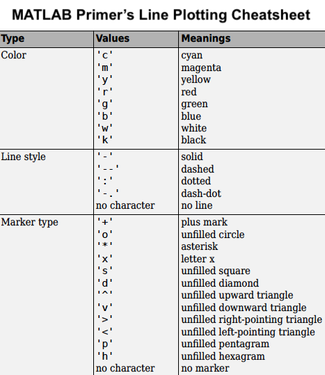 . Also if you scroll down to the bottom of the matplotlib.pyplot.plot page where the "Notes" for the page are.
#############################################
#
#  X-Y plot ...
#    with an red line
#
#     the "r" is changing the color of the line.
#     the online documentation gives you a set
#     of customizations that are available to you.
#

plt.plot(N_array,
         pi_of_N,
        'r')

#
#############################################

#############################################
#
#  X-Y plot...
#    with a blue dot-symbol for each point.
#

plt.plot(N_array,
         pi_of_N,
        '.b')

#
#############################################

#############################################
#
#  X-Y plot...
#    with a black o-symbol for each point.
#    and a solid line.
#

plt.plot(N_array,
         pi_of_N,
        'ok-')

#
#############################################

#############################################
#
#  X-Y plot...
#    with a green dashed line.
#

plt.plot(N_array,
         pi_of_N,
        'g--')

#
#############################################

#############################################
#
#  X-Y plot...
#    with a magenta plus-symbol for each point.
#    and a dotted line line.
#

plt.plot(N_array,
         pi_of_N,
        '+m:')

#
#############################################

Experiment with different options (It's your graph. Own it,)
Need to change axes?
Log-ing axes is done with specific formulas that use the same customization options as the simple linear plots.
- matplotlib.pyplot.semilogx - log-x linear-y
- matplotlib.pyplot.semilogy - linear-x log-y
- matplotlib.pyplot.loglog - both axes log-ed
#############################################
#
#  log-X-Y plot...
#    with a blue plus-symbol for each point.
#    and a dotted line line.
#

plt.semilogx(N_array,
             pi_of_N,
             'or:')

#
#############################################

Need more than one parameter plotted?
#############################################
#
#  X-Y plot...
#    with multiple series
#

plt.plot(N_array, pi_of_N - 0.1, 'ob:',
         N_array, pi_of_N,       'og:',
         N_array, pi_of_N + 0.1, 'or:')


#
#############################################

As we've been doing these you've noticed that the axes are not labled, nor are there titles, and especially in this case, nor is there a legend showing which series is which.
You've made a pretty graph. Don't get docked for not labeling it!
Here's how.
These need to be done with a separate command for each attrubute... as shown here:
#############################################
#
#  X-Y plot...
#    with an x- and y-axis label set.
#    including a title
#

plt.plot(N_array,
         pi_of_N,
        'or:')
plt.xlabel("Iterations (N)")
plt.ylabel("Estimated $\pi$")   # oooo look you can use LaTex Markup Here too!
plt.title("Estimating $\pi$ with Reimann Sums")
#
#############################################

And for our multiple series graph?
#############################################
#
#  X-Y plot...
#    with multiple series
#    ... and a legend
#

plt.plot(N_array, pi_of_N - 0.1, 'ob:',
         N_array, pi_of_N,       'og:',
         N_array, pi_of_N + 0.1, 'or:')
plt.xlabel("Iterations (N)")
plt.ylabel("Estimated $\pi$")   # oooo look you can use LaTex Markup Here too!
plt.title("Estimating $\pi$ with Reimann Sums")
plt.legend(["$\pi - 1$",
            "$\pi$",
            "$\pi + 1$"])

#
#############################################

If you want a solid line going through the graph, there is a painless way to do that, too.
- matplotlib.pyplot.hlines(y, xmin, xmax) - plot a horizontal line(s)
- matplotlib.pyplot.vlines(x, ymin, ymax) - plot a vertical line(s)
#############################################
#
#  X-Y plot...
#    with a reference horizontal line
#

plt.plot(N_array,
         pi_of_N,
        'or:')
plt.hlines(np.pi, 0, 20, 'm')
plt.xlabel("Iterations (N)")
plt.ylabel("Estimated $\pi$")   # oooo look you can use LaTex Markup Here too!
plt.title("Estimating $\pi$ with Reimann Sums")

#
#############################################

Things to Try
Once you are confortable with the plotting options for the x-y plots and their additional features (e.g., axes) explore the matplotlib gallery to see what other kinds of plottng are available with that package. There are also some sample tutorials as well as you become more ~reckless~ daring.
Deep Dive: Another way to Declare Plots
I used a very simple way to make graphs.
But if you start googling for support on how to make graphs in Python, you will frequently see the following syntax offered as a solution. This was one of the things that really confused me at first so I want to add this as a deep-dive.
This leverages the idea of "matplotlib.pyplot.subplots" that will let you use multiple plots in the same graphics space. If you scroll down on the above link to matplotlib.pyplot.subplots, you will see that these objects have their own modifiable attributes.
#############################################
#
#  X-Y plot using the fig/ax subplot method
#

fig, ax = plt.subplots()


ax.plot(N_array,
         pi_of_N,
        'or:')

ax.hlines(np.pi, 0, 20, 'm')

#
# Notice the new use of "set"
#

ax.set_xlabel("Iterations (N)")
ax.set_ylabel("Estimated $\pi$")
ax.set_title("Estimating $\pi$ with Reimann Sums")

#
#############################################
If you are making a plain simple plot the earlier method will likely work for you as you start Python.
But if you want to start getting fancy, there are a lot of things that the ax and fig attributes will do for you.
This is an example with a lot of comments and handholding to make a four-pannel plot.
(This is often far more work than I invest in making plots unless it's an automated process where I have to make a LOT of specialized plots.)
#############################################
#
#  Make a 2x2 plot with differennt logs on the
#    axes to demonstrate leveraging the ax-and-fig
#    method of plotting.
#
# We'll start by making a pair of x-ys.
#
#           x = array from 1-10
#           y = x - squared
#

x = np.arange(1,10+1)
y = x**2

#
# We'll start with the subplot command which
#    will let us make 2 rows (first argument)
#    and 2 columns.
#
# The second modifier pair instruct the matplotlib
#    "share" the axis attributes for each plot.
#
# When we do this, FIG will represent the atributes
#     of the whole plotting area.
#
# The acutal "subplots" are typically called "ax"
#     which you can consider to be the
#


fig, ax = plt.subplots(2,            # 2 rows in the y
                       2,            # 2 cols in the x
                       sharex='col', # set the colum (x axes to match)
                       sharey='row') # set the rows (y axes to match)

#
# We're going to arrange this as a 4-plot image with both
#    linear and log axes
#
# First Y [0,:] axis = Linear
# First X [:,0] axis = Linear
#
# Second Y [1,:] axis = Log
# Second X [:,1] axis = Log
#


#  Top Row
#  Y, X <- Row comes first
ax[0, 0].plot(    x, y, "g")  # Top Left (green)
ax[0, 1].semilogx(x, y, "k")  # Top Right (black)


#  Bottom Row
#  Y, X <- Row comes first
ax[1, 0].semilogy(x, y, "r")  # Bottom Left (red)
ax[1, 1].loglog(  x, y, "b")  # Bottom Right (blue)


#  Let's do the Y axis Labels -
ax[0, 0].set_ylabel("$x^2$")
ax[1, 0].set_ylabel("$x^2$ [logged axis]")

ax[1, 0].set_xlabel("x")
ax[1, 1].set_xlabel("x [logged Axis]")

#  And finally the title (the title here
#     is for the figture not any given
#     subplot)

fig.suptitle("Example of 2x2 Plot Area")

#
############################################

Version Information
################################################################
#
# Loading Version Information
#

%load_ext version_information

%version_information version_information, numpy, matplotlib

#
################################################################